Decision trees are a Supervised Machine Learning algorithm used to classify data. Decision Trees are very popular because they are effective and easy to visualize and interpret. Essentially, a decision tree is a flowchart where each level represents a different yes/no question. There are 3 different parts to a tree:
- Internal Nodes - each represents a ‘test’ on an attribute (i.e. does a coin flip end up heads or tail)
- Edges/Branches - the outcome of the test
- Leaf Nodes - predicts outcome by classifying data (this is a terminal node meaning there are no further nodes/branches)
As an example for how to use a decision tree, let’s say you want to play a game of soccer. In order to play outside, you need nice weather. A decision tree can be used to predict whether or not you can play soccer based on different weather features as shown below.
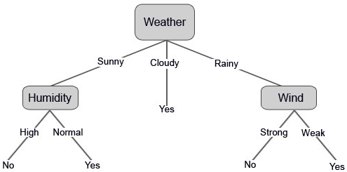
Source: https://www.educba.com/decision-tree-algorithm/
Here the internal nodes are questions such as ‘is it sunny, rainy, or cloudy?’ or ‘is there high humidity?’. The edges/branches are the answers bringing you to the next node (i.e. it is sunny or it is cloudy). And the leaf nodes are the yes and no at the bottom of the diagram telling you if you can play outside or not. So, the algorithm starts with the top question of ‘is it sunny, rainy, or cloudy?’ and makes a decision (a.k.a. the answer to the question). Then based off this decision, moves on to the corresponding next question. This continues until we have a final result and our data has been classified appropraitely.
Training Decision Tree:
It is important to train your decision tree in order to make sure that you are selecting the correct features to make a split on as this could effect the efficacy of the model. Training uses ‘recursive binary splitting,’ which considers all features and different split points are tried and tested based on a designated cost function. It selects the split with the lowest cost. The process to train data consists of:
- Use training dataset with features/predictors and a target.
- Make splits for the target using the values of predictors. Feature selection is used to determine which features to use as predictors.
- Grow tree until a stopping criteria is met.
- Show the tree a new set of features using an unkown class. The resulting leaf node is the class prediction for this example.
Creating a Decision Tree:
Let’s walk through an example of how to run a decision tree classifier using scikit-learn. For this example, I will be using a dataset containing information on Terry Stops. A terry stop is when a police officer stops a person based on ‘reasonable suspicion’ that the person may have been involved in criminal activity. We will be using this data to predict whether or not a terry stop ends in an arrest. Once all of the necessary pre-processing of the data has been done, we can begin by finding the best parameters to minimize our cost function. Trying different parameters is a great way to tune our algorithm. For decision trees, here are a few parameters to consider adjusting:
- DecisionTreeClassifier - measures the quality of the split using impurity measures such as ‘Gini’ or ‘Information Gain’.
- max_depth - how deep to make the tree. If ‘None’, nodes are expanded until all leaves are pure or until all leaves contain less than min_samples_split samples.
- min_samples_split - sets the minimum number of samples needed to split a node.
- min_samples_leaf - identifies minimum number of samples we want a leaf node to contain. Once achieved at a node, there are no more splits.
- max_features - number of features to consider when looking for the best split.
These are just a few of the many parameters you can set. Rather than having to try different combinations of these parameters individually, we can create a grid search function to run through all of the different combinations based off the parameter inputs we provide. To do so, we have to provide the classifier we want to use and the parameter inputs, as shown below.
# Determine optimal parameters:
# Declare a baseline classifier:
dtree = DecisionTreeClassifier()

# Create a parameter grid and grid search to identify the best parameters:
param_grid = {
    "criterion": ["gini", "entropy"],
    "max_depth": range(1,10),
    "min_samples_split": range(2,10)
}
gs_tree = GridSearchCV(dtree, param_grid, cv=5, n_jobs=-1)

# Fit the tuned parameters:
gs_tree.fit(X_train_ohe, y_train)

# Print best estimator parameters:
print(gs_tree.best_params_)
Running this function told us that the best parameters based on the inputs we provided are a gini criterion with max_depth = 1 and min_samples_split = 2. Once we have this info, we can go ahead with creating our decision tree classifier using these parameters. We then fit the model to the training data and predict the testing data.
# Create the classifier, fit it on the training data and make predictions on the test set:
d_tree = DecisionTreeClassifier(criterion='gini',max_depth=1,min_samples_split=2)
d_tree = d_tree.fit(X_train_ohe, y_train)
y_pred = d_tree.predict(X_test_ohe)
Now that we have our algorithm run, we need to pull a few metric to determine how well our model has performed. There are 2 different variables I am going to look at. The first is the accuracy score. This tells you how accurate your classification model is.
print('Decision Tree Accuracy: ', accuracy_score(y_test, y_pred)*100,'%')
We get an accuracy score of 79.95872884853488 %. Meaning, our model can correctly predict when an arrest was made from a terry stop 79.96% of the time. I then look at a confusion matrix. A confusion matrix is a table used to describe the performance of a model, and it is a good way to visualize how accurate our model is. The confusion matrix will show us how many of each of the below groupings the model gives us:
- True Positives (TP) - # of observations where model predicted person was arrested and they actually were arrested
- True Negatives (TN) - # of observations where model predicted person was not arrested and they actually were not arrsted
- False Positive (FP) - # of observations where model predicted person was arrested but they are actually were not arrested
- False Negative (FN) - # of observations where model predicted person was not arrested and the actually were arrested
Below is a function that can be used to create a confusion matrix:
# Define Confusion Matrix:
def confusion_matrix_plot(cm, classes,
                          normalize=False,
                          title='Confusion matrix',
                          cmap=plt.cm.Blues):
    '''This function will create a confusion matrix chart which shows the accuracy breakdown of the given model.
    Inputs:
    cm: confusion matrix function for tested and predicted y values
    classes: variables to identify for each class (0 or 1)
    normalize: if True will normalize the data, if False will not normalize the data
    title: title of the chart
    cmap: colors to plot
    '''

    plt.imshow(cm, interpolation='nearest', cmap=cmap)

    # Add title and labels:
    plt.title(title)
    plt.ylabel('True label')
    plt.xlabel('Predicted label')

    # Add axis scales and tick marks:
    tick_marks = np.arange(len(classes))
    plt.xticks(tick_marks, classes, rotation=45)
    plt.yticks(tick_marks, classes)

    # Add labels to each cell:
    thresh = cm.max() / 2.
    # Iterate through confusion matrix and append labels to the plot:
    for i, j in itertools.product(range(cm.shape[0]), range(cm.shape[1])):
        plt.text(j, i, cm[i, j],
                 horizontalalignment='center',
                 color='white' if cm[i, j] > thresh else 'black')

    # Add legend:
    plt.colorbar()
    plt.show()
Now to run this matrix:
# Use Arrested and Not Arrested for 0 and 1 classes
class_names = ['Arrested','Not Arrested']
# Confusion Matrix for Decision Tree
cm_dtree = confusion_matrix(y_test,y_pred)
confusion_matrix_plot(cm_dtree, classes=class_names, title='Decision Tree Confusion Matrix')

We see here that we have over 9,000 true positives (top left corner) and over 400 true negatives (bottom right corner). However we do have over 2000 incorrect classifications (bottom left and top right corners), indicating there is still room to improve this model.